The theme for the third week of Research Data and Digital Scholarship Data Jam 2021 was “Visualizing Text and Networks”.  

The “Network Visualization with R” workshop was a live-coding session which detailed the following: 

1. Glossary of Network Visualization Terms 

2. Software and Programming Alternatives to Network Visualization with igraph and NetworkD3 

3. Resources 

The R and RStudio demonstration included: 

• Nodes & Edges 

• Directed & Undirected Graph 

• Static and Dynamic Graphs 

• Customizations with layout, colors, & size 

Here is the link to the Video Recording of the Workshop.

Here is the link to the workshop materials including the R exercise code, completed exercise PDF, and Philadelphia Historical Streets Dataset used in the exercise.

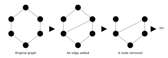
Network visualization allows the viewer to understand a lot of information quickly and intuitively about the state of the network at a glance. Social networks have actors with relations between them. Network diagrams (or Graphs) show interconnections between a set of entities. Each entity is represented by a Node (or Vertice). Connections between nodes are represented by links (or edges). 

R Packages commonly used for network visualization include: 

•  igraph: data preparation and plotting 
  • https://igraph.org/r/ 
• ggraph: plotting using the grammar of graphic 
  • http://users.dimi.uniud.it/~massimo.franceschet/ns/syllabus/make/ggraph/ggraph.html
• networkD3: interactive graphs
  • https://christophergandrud.github.io/networkD3/

Other relevant R Packages include: 

• Static Network Visualization: 

  • igraph 

  • ggraph 

  • network 

  • sna 

  • threejs 

  • ndtv 

  • statnet 

  • ggiraph 

• Dynamic Network Visualization: 

  • networkD3 

  • VizNetwork 

The Python library alternatives are: 

• NetworkX 

• igraph 

The Julia library alternatives: 

• JuliaGraph 

Software alternatives for network visualization are: 

• Gephi

• Cytoscape 

• Palladio 

• Pajek 

For the RStudio demonstration, after installing and running igraph package, a variety of graphs were displayed.  

# Install igraph library 

install.packages("igraph") 

# Run igraph library 

library(igraph) 

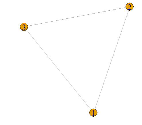
These included graphs with different number of nodes and edges, directed and undirected graphs, and graphs of different shapes. For example:

# Create a directed graph with 3 nodes 1, 2, and 3 

g3d <- graph( edges=c(1,2, 2,3, 3, 1), n=3, directed=T)  

plot(g3d) 

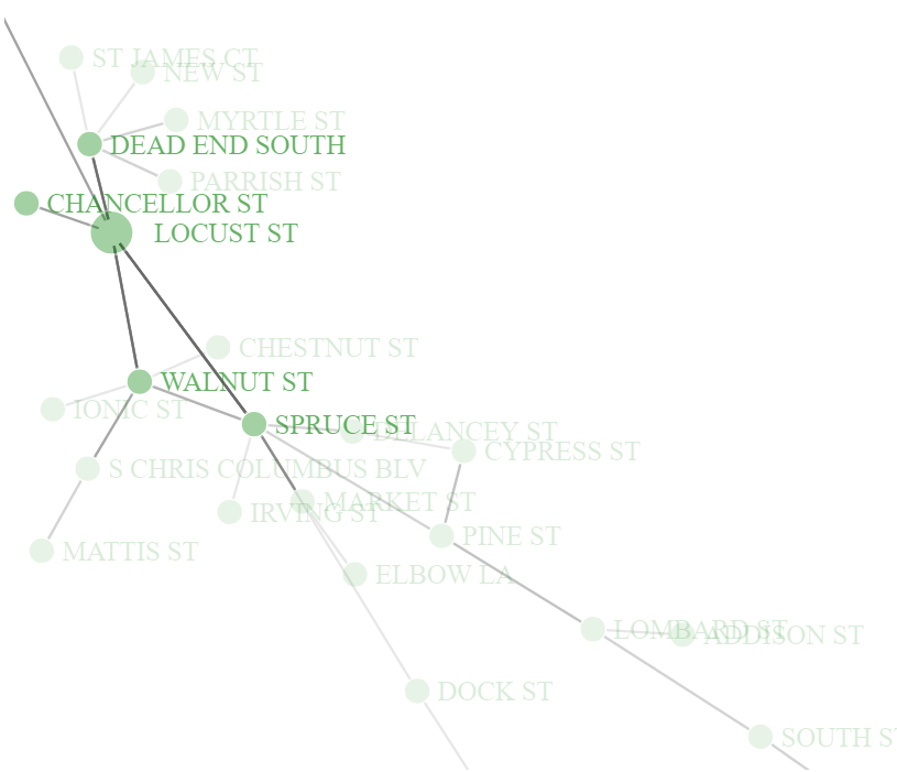
A simple graph was developed in the form of visualizing a network of historical roads in Philadelphia where the starting point of a street and the ending point of the street are the source and destination, respectively.  

## Interactive Network Graphs 

## Historic Streets of Philadelphia 

         library(networkD3) 

# Load data 

          edges <- read.csv("Historic_Streets.csv") 

          head(edges) 

          # Identify Source and Target Edges 

           source <- edges["FROM_STREET"] 

                     target <- edges["TO_STREET"] 

# Format into network data 

                     networkData <-data.frame(source, target)   

           simpleNetwork(networkData, nodeColour= "green", zoom=T,  

                                                       height = 300, width = 300, fontSize = 16) 

The network of interactions in the book Les Misérables by Victor Hugo was also mapped as a force-directed network graph. 

## Network of Interactions in Les Miserables characters 

# Load data 

         data(MisLinks) 

         data(MisNodes) 

  

head(MisNodes) 

         head(MisLinks) 

  

# Plot 

forceNetwork(Links = MisLinks, Nodes = MisNodes, 

                                       Source = "source", Target = "target", 

                              Value = "value", opacityNoHover = 0.9, NodeID = "name", 

                                        Group = "group", opacity = 0.8, zoom=T) 

# Find all links to Valjean 

         which(MisNodes == "Valjean", arr = TRUE)[1] - 1 

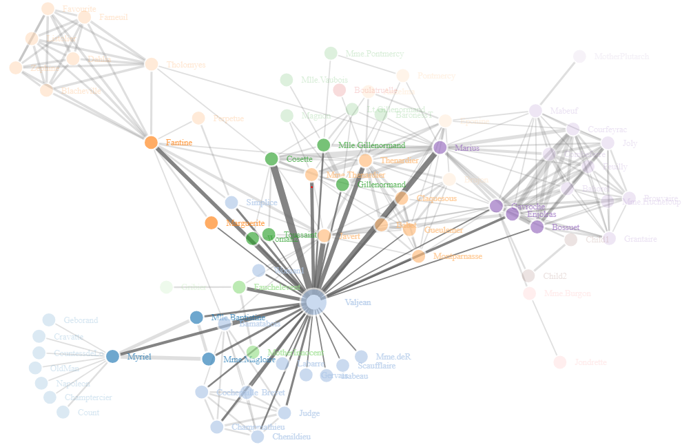
This graph shows the network of character interactions occurring across the novel at a glance.

Finally, a study of Zachary’s Karate Club Network helped learners understand the use-case of Network Analysis beyond network visualization. 

## Zachary's Karate Club Network  

library(igraphdata) 

          data(karate) 

head(karate) 

# How many factions are in the karate club? 

plot(karate) 

# How many subcommunities clusters are in the karate club? 

cfg <- cluster_fast_greedy(karate) 

          plot(cfg, karate) 

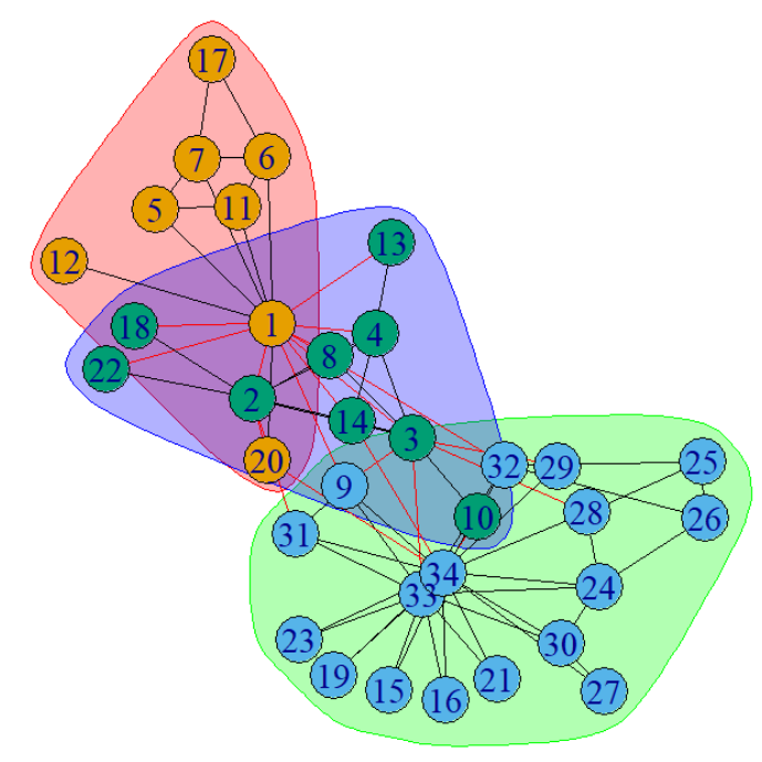
This graph represents the three major communities and sub-communities within in the network.

It is important to keep in mind the accessibility concerns of network visualizations. For example, overlapping nodes might make the graph seem populated with lower number of nodes. While changing the size and color of nodes might be helpful to discern or distinguish the types of nodes, it might lead to confusion. The 2D graph might be mistaken for occupying 3D space. It is also helpful to use the ColorBrewer2 app to confirm the accessibility features of the colors used in the graph.

Other ways to distinguish nodes, edges, clusters, and networks are as following:

# nodes/vertices: color, shape, size, border, labels ,text-size, position 

# edges/links: color, size, labels, arrows, curvature, link distance 

# groups/communities: color, shading, border, lines 

# graph: layout, color, faceting 

Resources: 

• Static and dynamic network visualization with R, Katya Ognyanova, https://kateto.net/ 

• Network Visualization Basics with NetworkX and Plotly in Python, Rebecca Weng, https://towardsdatascience.com/tutorial-network-visualization-basics-with-networkx-and-plotly-and-a-little-nlp-57c9bbb55bb9 

• UPenn LibGuide on Social Network Analysis, Lauris Olsen, https://guides.library.upenn.edu/sna 

• Network Analysis Using R, Yunran Chen, https://yunranchen.github.io/intro-net-r/ 

• Temporal Network Visualization Example, http://curleylab.psych.columbia.edu/netviz/netviz5.html#/25 

• Six Degrees of Francis Bacon (Carnegie Mellon), http://www.sixdegreesoffrancisbacon.com/?ids=10000473&min_confidence=60&type=network 

• Awesome Network Analysis Github Masterdoc, https://github.com/briatte/awesome-network-analysis 

• Network R Graph Gallery, https://www.r-graph-gallery.com/network.html 

Terminology 

• Brian V. Carolan, “Key Terms,” Social Network Analysis and Education: Theory, Methods & Applications (SAGE, 2014, http://www.sagepub.com/carolan/study/materials/KeyTerms.pdf); 

• Datavu, “Introduction to Network Analysis terminology” (http://datavu.blogspot.com/2013/10/sna-social-network-analysis-basic.html); 

• Katharina Zweig, “An Introductory Course on Network Analysis” (https://sites.google.com/site/networkanalysisacourse/schedule/an-introduction-to-centrality-measures).